Observable Machine Learning Models for Shogun (Part 1)
Introduction
Shogun is a machine learning framework which provides efficient implementations of the most common algorithms to solve large-scale problems. The toolbox is completely written in C++ and it offers several interfaces in other languages as well (e.g. python, Java, Javascript, etc.).
Since Shogun is one of the oldest available machine learning frameworks (its development started in 1999), in the past few years it has undergone an extensive development effort such to update and improve its internal structure.
With this in mind, we also started to work on the usability of the toolbox itself. In particular, we wanted to make more transparent Shogun’s internal models by making them emit data while they are running. Currently, once a call to the train() method is issued, it is not possible to see anymore the internals of a model. Therefore, the final users are basically looking at a “black box”, an opaque machine in which they cannot identify its inner workings.
For instance, when we use Shogun’s cross-validation to validate our machine learning models, it is hard for us to extract information from each of the fold runs. For instance, we might be interested in inspecting the machine trained at a certain fold. These kind of goals are usually not possible (or not straightforward to achieve).
Let’s look at another example. Imagine that we are training a simple classifier using the Perceptron model. We might be interested in seeing how the hyperplane changes while we are fitting the model. With current ML frameworks, it is hard to accomplish such task.
The Project
This is the first post of a series which documents the work we are currently doing on the Shogun’s library such to improve and apply the new observer infrastructure codebase-wise. These new features would help in making Shogun’s models more understandable to the final users.
These efforts started in 2017 when I implemented the basic framework during the Google Summer of Code. However, the architecture was still at its early stage and therefore was not employed effectively inside Shogun. Now it is time for it to be used and finalized.
The project is divided roughly into four main tasks:
- Modernize the observable architecture and improve its general structure;
- Upgrade Shogun’s algorithms by making them emit key values during training;
- Write new parameter observers which will exploit the new observable algorithms;
- Provide a couple of real-world applications of these two features.
This blog post will cover mostly the work done for the first point of the list presented above and it will also show the result obtained.
Architecture Overview
The architecture is pretty simple and it only has three main components:
- A method which is used to emit values;
- A construct which will work as a wrapper around the values we want to emit;
- Parameter observers which will received the values from the various machines;
We employed the Observer Pattern to make all Shogun’s algorithms observable. This design pattern is mainly used to implement an event-handling system in which a subject maintains a list of observers and notifies them automatically of any state change.
More specifically, in Shogun each model has a subscribe() method which a ParameterObserver object can use to get information from the given model. A Shogun’s model also has another method called observe() which can be used to transmit information to all the attached observers. The observe() method is for internal use only and it is not exposed.
We did not implement the observer pattern ourselves. We used instead RxCpp which is a header-only C++ library that offers several algorithms for building asynchronous and event-based programs.
ObservedValue and ObservedValueTemplated
What kind of information is passed to the observers? Virtually, any object can be emitted by the models to the various observers. In order to provide this flexible functionality, we implemented a “wrapper” class, called ObservedValue, which can be used to store efficiently any data that a model may want to send around.
Since we used the new get()/put() methods from Shogun, we had to provide a typed wrapper (such to store whichever object needed). That is easily achievable by using C++ templates. However, we also needed to provide a clear interface to create/emit these ObservedValue. We then split the template functionality such to build two classes. The final architecture was the following:
class ObserverdValue : public CSGObject
{
    // It is basically an empty class which provides only get() and put()
    // methods.
};

template <class T>
class ObservedValueTemplated : public ObservedValue
{
    template <class T>
    ObservedValueTemplated(T value) : ObservedValue(), m_value(value);

private:
    T m_value;
};
In order to observe something, an ObservedValueTemplated object is generated. Moreover, thanks to inheritance mechanisms, the observer works only with ObservedValue objects. This simplifies the overall API and it preserves the intended functionalities. In order to retrieve the observed value we just need to call the appropriate getter:
ObservedValue obs;
obs.get<type>("name_of_the_stored_parameter");
A simple observable model
As a simple example, we will build a binary classifier using as a model the AveragedPerceptron. Moreover,
we will use Shogun’s Python interface to code it.
First of all, we import some Shogun’s methods which will be used to instantiate
the various objects and algorithms (we could also write import shogun as sg and
use all methods by as sg.csv_file, sg.features and so on).
from shogun import csv_file, features, labels, machine, parameter_observer
Then we load the data files which contains the features and labels needed for this example. You can download these files from here:
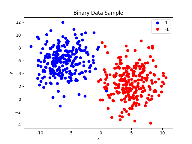
It is a small dataset (1000 samples) composed by two dimensional points which can have two labels -1 and 1.
f_feats_train = csv_file("classifier_binary_2d_linear_features_train.dat")
f_feats_test = csv_file("classifier_binary_2d_linear_features_test.dat")
f_labels_train = csv_file("classifier_binary_2d_linear_labels_train.dat")
f_labels_test = csv_file("classifier_binary_2d_linear_labels_test.dat")

features_train = features(f_feats_train)
features_test = features(f_feats_test)
labels_train = labels(f_labels_train)
labels_test = labels(f_labels_test)
The data are linearly separable, as we can see from the plot below.
We then initialize the model and we attach a parameter observer to it. In this example, we use a logger which will print all the information it receives on stdout.
perceptron = machine("AveragedPerceptron", labels=labels_train, learn_rate=1.0, max_iterations=1000)

observer = parameter_observer("ParameterObserverLogger")
perceptron.subscribe(observer)
We then train our model and we apply it to the test features.
perceptron.train(features_train)
labels_predict = perceptron.apply(features_test)
We are pretty much done! Once we run this code, the output will be something similar to this:
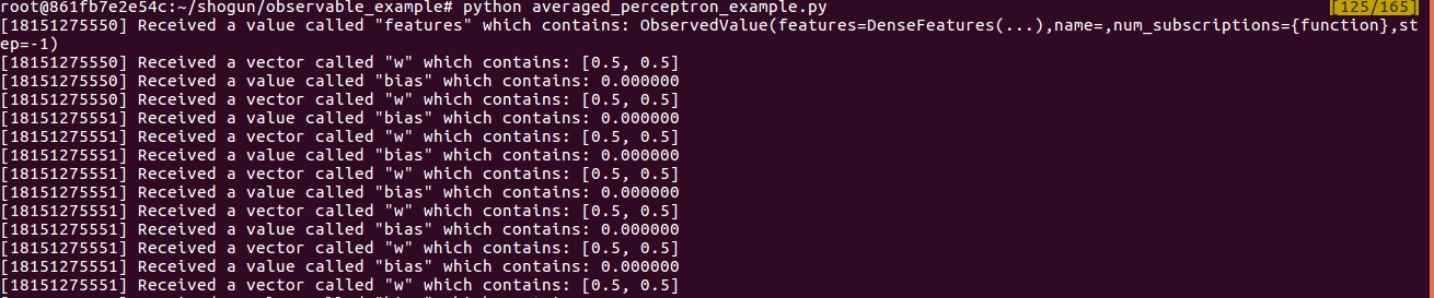
As you can see, the AveragedPerceptron emits its weights and bias.
By looking at them we can get a certain idea about how the hyperplane is changing
(if we are in a low dimensional space) and we can use those data to build nice
visualizations. For instance, by adding more python code we can generate a nice
video in which we show how the separation plane changes during training.
#
# Code for producing the animation
#
import matplotlib
matplotlib.use('Agg')
from matplotlib import pyplot as plt
from matplotlib import animation
import numpy as np

fig = plt.figure()
ax = plt.axes()
line, = ax.plot([], [])

plt.suptitle("Binary Data Sample")

# We first need to divide the samples into the two classes (-1 and 1).
# We will use four lists to store their x and y coordinates.
blue_x = []
red_x = []
blue_y = []
red_y = []

for i in range(0, features_train.get_num_vectors()):
    mat = features_train.get("feature_matrix")
    if (labels_train.get("labels")[i] == 1):
        blue_x.append(mat[0][i])
        blue_y.append(mat[1][i])
    else:
        red_x.append(mat[0][i])
        red_y.append(mat[1][i])

# Filter the observations by looking only at bias and weights.
# We also store them into two lists to make things easier.
w = []
bias = []
for i in range(0, observer.get("num_observations")):
    if (observer.get_observation(i).get("name") == "w"):
        w.append(observer.get_observation(i).get("w"))
    elif (observer.get_observation(i).get("name") == "bias"):
        bias.append(observer.get_observation(i).get("bias"))

# This function will be used to initialize the first frame of the
# video. We just plot the two classes and we set some labels.
def init():

    plt.plot(blue_x, blue_y, 'bo', label="Label = 1")
    plt.plot(red_x, red_y, 'ro', label="Label = -1")

    line.set_data([], [])
    line.set_label("hyperplane")

    plt.xlabel("x")
    plt.ylabel("y")

    return line,

# This function will be called for each observation (from i to len(w)).
# Each time we compute the hyperplane by looking at the bias and weights.
def animate(i):
    print("Processing observation: {}/{}".format(i, len(w)))
    plt.title("Iteration {}".format(i))
    x = np.linspace(-10, 10, 1000)
    line.set_data(x, x*w[i][0]+x*w[i][1]+bias[i])

    return line,

# Run the actual animation call which will generate the video.
anim = animation.FuncAnimation(fig, animate, init_func=init, frames=len(w), interval=200, blit=True)
anim.save('./video/hyperplane.mp4', fps=30, extra_args=['-vcodec', 'libx264'], bitrate=500)
We can see the result below. The separation plane changes from its initial position to the one which minimize the classification error.
Conclusions
Now that the architecture is finalized, the next steps will be to apply it to the Shogun’s models. This will be done by updating their train() method such to emit valuable information while they are being fitted. For instance, as we did for the AveragedPerceptron example, the new observable models will be able to emit their weights and biases during training to give to the users valuable new insights.
The final goal will be making the users able to build their machine learning models with interactive
visualizations which will provide a concrete real-time feedback.
Useful links
If you need more technical informations, please refer to the links provided below. Have a look to the various PRs to see which was the development process and what were the features implemented.
Code
The complete code for the example shown above can be found here.
Be aware that, in order to run it. you would need to have compiled manually Shogun since these
features are still experimental and therefore are not part of an official release.
All these features can be found in the following branch feature/observable_framework.